NEB calculation

0.2 Theoretical Background

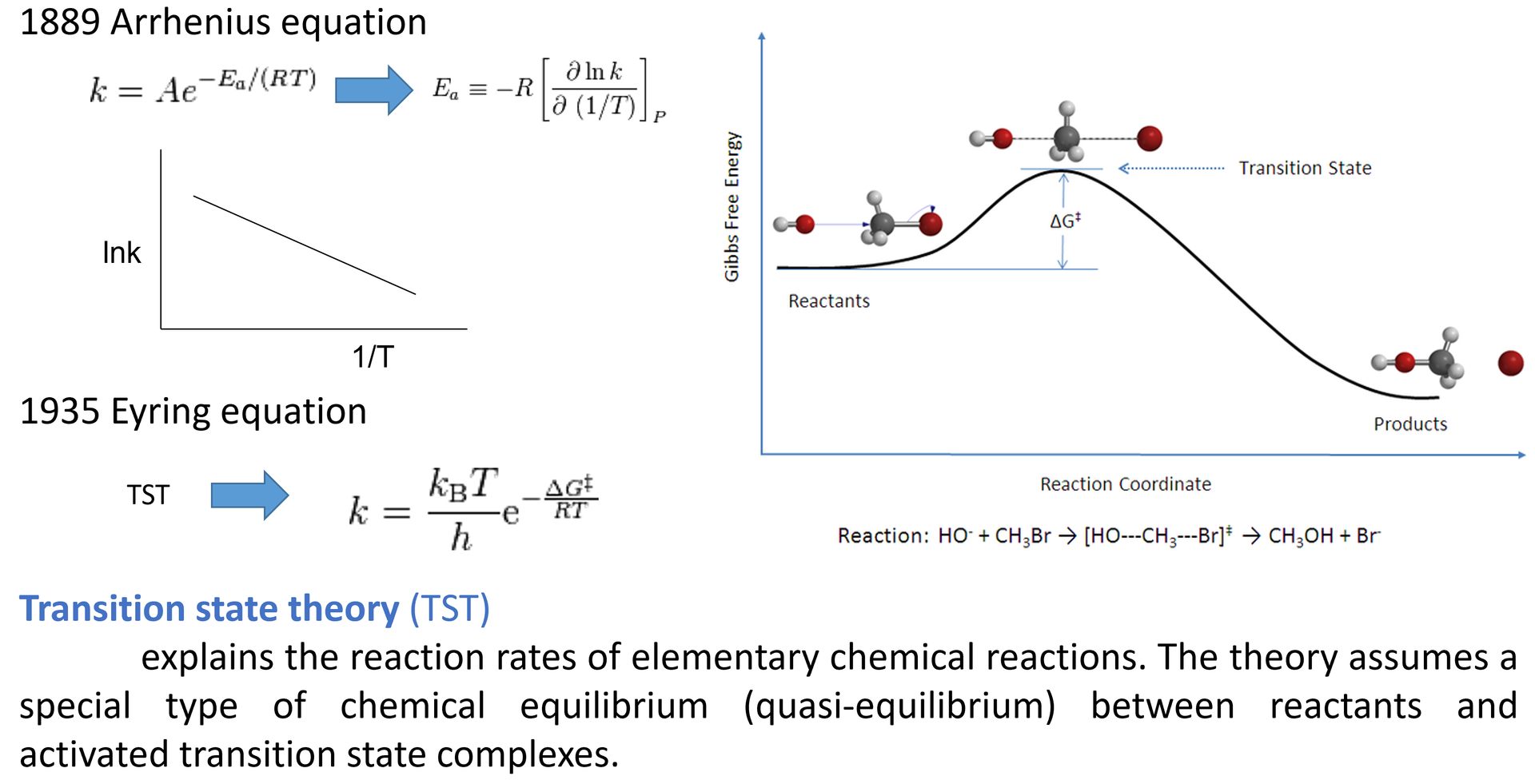
0.2.1 Transition-State Theory

Transition-state search aims to locate and optimize a first-order saddle point. This point is the highest-energy point along the minimum-energy path (MEP), while it is a minimum with respect to all directions perpendicular to the MEP.

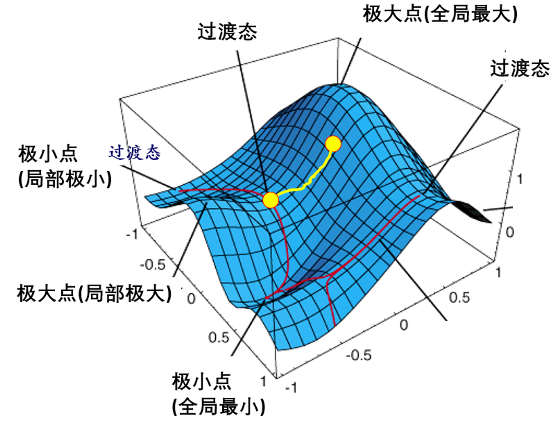
The transition state can be pictured as the mountain pass between two valleys:

When climbing between two valleys, the minimum-energy route generally passes through the intermediate mountain pass.

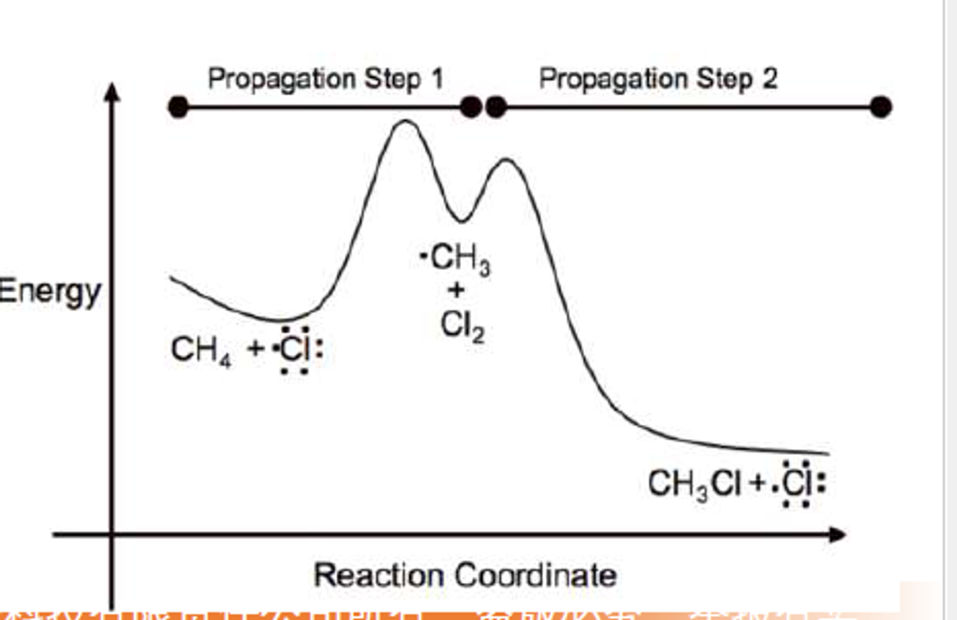
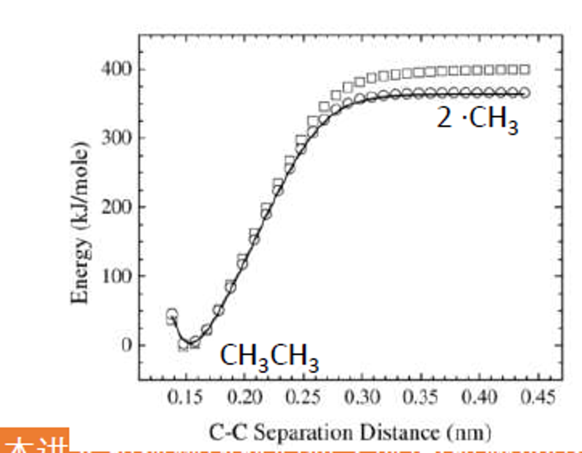
Not every chemical process has a well-defined transition state in a static potential-energy calculation. Examples include:

• Ionic dissociation into cations and anions, or recombination of cations and anions.



• Covalent-bond cleavage into two radicals, or radical recombination.



• Some surface adsorption and desorption processes.
• Some adsorption or desorption processes do not show a transition state in a static calculation, but a transition state may exist on the free-energy surface obtained from finite-temperature simulations. This difference is an entropic effect.

The importance of the transition state is expressed by the Eyring equation:

$
k = \frac{k_B T}{h}\exp\left(-\frac{\Delta G^{\ddagger}}{RT}\right)
$

Here, $k$ is the reaction rate constant and $\Delta G^{\ddagger}$ is the activation free energy.

NEB Principles

NEB Principles and Steps: The NEB (Nudged Elastic Band) method can be understood as a string of beads connected by springs: beads are placed sequentially between initial valley A and final valley B, with heights positioned by linear interpolation. Intuitively, if released directly, all beads would roll back to the valley bottoms. However, springs connecting adjacent beads prevent complete dispersion while allowing each bead to slide downhill under perpendicular forces. Through iterative optimization, the bead chain settles along the lowest energy route connecting A and B. This determines the minimum energy path between valleys while estimating the barrier crossing energy.

Each image is subject to two types of force:

1. The true force from the potential-energy surface.
2. The spring force, which maintains the spacing between neighboring images.

• Algorithm Steps (pseudocode):

1. Initialize Path: Load initial configuration A and final configuration B, generate intermediate configurations as "images" (typically through linear interpolation; 3-5 images for simple reactions, 10+ for complex processes).

1. Connect Springs: Link adjacent image pairs with virtual springs having zero natural length (tendency to pull images together). Initial and final states remain fixed as endpoints; other images participate in optimization vasp.atvasp.at.

1. Calculate Net Force: For each intermediate image, compute two components: spring force along the path tangent (pulling images toward neighbors) and potential surface force with only the perpendicular component retained (tangential components are projected out to prevent sliding into valleys) 3d-materials-lab.gitbook.io. Net force = spring force (parallel) + potential force (perpendicular) mattermodeling.stackexchange.com.

1. Update Positions: Move each intermediate image along its net force direction using optimization algorithms (conjugate gradient, steepest descent). Motion is constrained to maintain path ordering.

1. Check Convergence: Iterate steps 3-4 until forces approach zero or fall below threshold and position changes are minimal. The path is considered converged with all images on the approximate minimum energy path.

1. Output Results: Record energies for each converged image. Plot energy vs. reaction coordinate to obtain the reaction barrier (highest energy difference). Higher resolution sampling can be performed by adding images if needed.

• Common Issues/Troubleshooting:

• Image Count: Too few images may miss path details or fail to locate the maximum accurately; too many increase computational cost and may introduce oscillations. Start with 3-5 images for simple reactions, increasing to 10+ for complex paths. Persistent convergence failure usually indicates insufficient images 3d-materials-lab.gitbook.io.

• Spring Stiffness: Use moderate spring constants (e.g., VASP default -5 for automatic adjustment). Weak springs cause clustering near potential wells; strong springs deviate from true MEP. Default values typically work well vasp.at.

• Initial Path: NEB depends on initial path quality. Poor initial interpolation may converge to unreasonable local paths. Try manually adjusting intermediate configurations or segmented NEB with known intermediate states.

• Drift and Algorithms: All images optimize simultaneously, potentially causing drift if translational/rotational degrees of freedom exist. Programs typically subtract this drift. NEB's constrained optimization requires robust optimizers rather than simple conjugate gradient. For convergence difficulties, try different algorithm parameters (e.g., VASP IBRION=3 fast damping vasp.at).

Climbing Image NEB

CL-NEB Principles and Steps: Climbing-Image NEB (CI-NEB) adds a refinement step after standard NEB convergence to precisely locate the transition state (MEP highest point). Standard NEB yields only approximate transition states, as the highest energy image may deviate from the true saddle point with limited image resolution. CI-NEB addresses this by "pushing" the highest image.

• Key Concept: Identify the current path's highest energy image and enable "unrestrained climbing." Specifically, remove spring constraints (no neighboring spring pulling) and reverse the real force along the band direction vtstools.readthedocs.io. Analogy: the highest bead was constrained by springs on both sides; now we cut the strings and reverse gravity, so instead of falling it gets "pushed" toward higher energy. This image climbs upward along the path tangent while stabilizing downward perpendicularly, moving toward the saddle point (highest along path, stable laterally) vtstools.readthedocs.iomattermodeling.stackexchange.com.

• Algorithm Steps:

1. Preliminary NEB: Run standard NEB until path roughly converges or takes shape. Don't enable climbing initially, as rough initial paths cause uneven distribution or deviation vtstools.readthedocs.io.

1. Enable Climbing Image: Identify the highest energy intermediate image in NEB results. Set its spring force to zero (cutting neighbor connections) and reverse its potential surface force component along the path direction vtstools.readthedocs.io. This image experiences "uphill" pushing along the reaction coordinate while maintaining downhill pull perpendicularly, promoting saddle point-only movement.

1. Iterative Optimization: Other images continue standard NEB optimization while only the climbing image follows modified forces. The climbing image gradually ascends to higher energies without neighbor pulling, precisely targeting the peak. Adjacent images may retreat slightly as the highest image no longer participates in spring-based spacing—this is normal vtstools.readthedocs.io.

1. Convergence Criteria: The climbing image reaches the saddle point when its net force approaches zero, especially along the path direction, and it represents an energy maximum (neighboring images have lower energies). This indicates a first-order saddle point position. Other images distribute along the MEP on both sides.

1. Record Transition State: Output the climbing image's configuration and energy as the transition state (saddle point structure and potential). Transition state energy is now more accurate than pre-climbing estimates.

• Common Issues/Troubleshooting:

• Climbing Timing: Never enable climbing image initially vtstools.readthedocs.io. First obtain a reasonable path with the highest image near the saddle point, then enable climbing for precise positioning. Premature climbing causes excessive upward movement and imbalanced distributions. Typical workflow: initial NEB convergence → enable climbing → reconverge.

• Single Peak Climbing: Usually enable climbing for only the single highest image. For multi-barrier systems, handle segments separately rather than simultaneous climbing, as force interactions become complex.

• Subsequent Refinement: CI-NEB transition states can be further validated with refined methods (reaction coordinate interpolation, separate TS optimization). However, CI-NEB typically provides sufficient accuracy for most systems.

DIMER method

Dimer Method Principles and Steps: The dimer method finds saddle points without requiring final states, making it ideal when reaction products are unknown or exploring various possible transitions ase-lib.org. The analogy is finding mountain passes on hillsides: standing in an energy valley surrounded by slopes, hoping to locate which direction leads to passes (saddle points) to other valleys. The dimer method uses a "tool"—the dimer (two very close configurations from small perturbations)—as probes that rotate and move on the energy surface to locate saddle point directions.

• Key Concept: The dimer method uses two nearly overlapping configurations to estimate potential energy surface curvature information. Visualize a short "dumbbell" on the potential surface with one end near the initial configuration and the other slightly offset. The algorithm rotates this dumbbell around its center, testing energy changes in different orientations to find the orientation giving lowest energy—indicating minimum curvature (flattest slope or downhill) chemistry.stackexchange.com. Minimum curvature directions typically correspond to "easiest uphill" directions (slowest descent or fastest ascent), pointing toward saddle points. Once determined, the dimer climbs forcefully in this direction while minimizing energy in perpendicular coordinates (ensuring no track deviation while climbing) manual.q-chem.com. Alternating rotation and movement gradually approaches the saddle point.

Note

Some online discussions claim that adding more CI-NEB images is always better. This is incorrect. Because the highest-energy image can climb automatically, even one intermediate image can sometimes locate the transition state accurately. In most cases, three or four intermediate images are sufficient for a normal transition-state calculation. The appropriate number of images should be estimated with the dist.pl script.

0.2.5 DIMER Method

The Dimer method is a transition-state search method that does not require prior knowledge of the final state and does not explicitly construct the Hessian matrix. It is particularly useful for finding a nearby saddle point from a known configuration, such as the transition state for the diffusion of an adsorbed atom on a surface. Unlike NEB, which requires both an initial state and a final state, the Dimer method requires only an initial configuration and a suitable initial perturbation direction. It therefore searches for a nearby saddle point accessible from the chosen initial configuration.

A dimer consists of two points that are very close to each other in configuration space. It can be viewed as a dumbbell oriented along the unit vector $\mathbf{n}$. Let the two endpoints be $\mathbf{R}+$ and $\mathbf{R}-$, let their midpoint be $\mathbf{R}$, and let the half-separation be $\Delta R$:

$
\mathbf{R}_\pm=\mathbf{R}\pm\Delta R\,\mathbf{n},
\qquad \|\mathbf{n}\|=1.
$

The distance between the two endpoints is $2\Delta R$. In practical calculations, $2\Delta R$ is usually very small, for example approximately $0.01\ \text{\AA}$. Denote the endpoint energies and forces by $E\pm$ and $\mathbf{F}\pm$, respectively, where

$
\mathbf{F}\pm=-\nabla E(\mathbf{R}\pm).
$

Because the dimer separation is small, the method is sensitive to force accuracy, electronic self-consistency, and the finite-difference step. A sufficiently tight electronic convergence criterion should therefore be used. For example, some VASP-VTST calculations use EDIFF = 1E-7, but the appropriate value should be tested for convergence according to the system size, exchange-correlation functional, and target force tolerance.

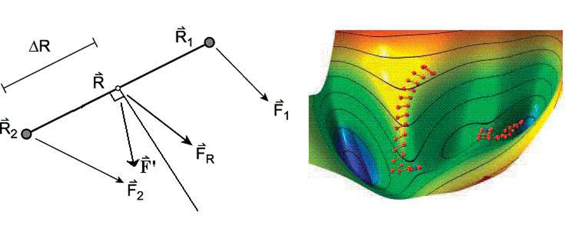
1. Midpoint, Average Energy, and Midpoint Force

The average endpoint energy and average endpoint force are defined as

$
\bar{E}(\mathbf{R},\mathbf{n})=\frac{E++E-}{2},
$

$
\mathbf{F}(\mathbf{R})=\frac{\mathbf{F}++\mathbf{F}-}{2}.
$

Expand the endpoint energy in a Taylor series around the midpoint $\mathbf{R}$:

$
E(\mathbf{R}\pm\Delta R\mathbf{n})
=E(\mathbf{R})
\pm\Delta R\,\nabla E(\mathbf{R})\cdot\mathbf{n}
+\frac{\Delta R^2}{2}\mathbf{n}^{\mathsf T}\mathbf{H}(\mathbf{R})\mathbf{n}
+O(\Delta R^3),
$

where $\mathbf{H}(\mathbf{R})=\nabla^2E(\mathbf{R})$ is the Hessian matrix of the potential-energy surface. Adding the two endpoint expansions cancels the first-order terms, giving

$
\bar{E}(\mathbf{R},\mathbf{n})
=E(\mathbf{R})
+\frac{\Delta R^2}{2}\mathbf{n}^{\mathsf T}\mathbf{H}(\mathbf{R})\mathbf{n}
+O(\Delta R^4).
$

Define the directional curvature along the dimer direction $\mathbf{n}$ as

$
C(\mathbf{R},\mathbf{n})
=\mathbf{n}^{\mathsf T}\mathbf{H}(\mathbf{R})\mathbf{n}.
$

Therefore, for a fixed midpoint and sufficiently small $\Delta R$,

$
\bar{E}\approx E(\mathbf{R})+\frac{\Delta R^2}{2}C(\mathbf{R},\mathbf{n}).
$

This shows that, during dimer rotation, the orientation dependence of the average endpoint energy primarily reflects the change in directional curvature. Strictly speaking, the algorithm is not searching for the minimum physical energy at a fixed midpoint; it is searching for the minimum directional curvature. Near a transition state, the minimum-curvature direction usually corresponds to the eigenvector of the Hessian with the lowest eigenvalue, namely the imaginary-frequency mode.

The average force satisfies

$
\mathbf{F}(\mathbf{R})
=\frac{\mathbf{F}++\mathbf{F}-}{2}
=-\nabla E(\mathbf{R})+O(\Delta R^2).
$

Thus, the average endpoint force provides a second-order approximation to the true force at the midpoint.

2. Finite-Difference Expression for the Curvature

The directional curvature can be estimated from the difference between the endpoint forces. From

$
\mathbf{F}--\mathbf{F}+
\approx 2\Delta R\,\mathbf{H}(\mathbf{R})\mathbf{n}
$

we obtain

$
C(\mathbf{R},\mathbf{n})
\approx\frac{(\mathbf{F}--\mathbf{F}+)\cdot\mathbf{n}}{2\Delta R}.
$

Alternatively, using the endpoint energies and the midpoint energy, the curvature can be written in central finite-difference form:

$
C(\mathbf{R},\mathbf{n})
\approx\frac{E+-2E(\mathbf{R})+E-}{\Delta R^2}.
$

In practice, the Dimer method usually estimates the curvature from forces because the force information is already available from the electronic-structure calculation at each endpoint, and no full Hessian needs to be computed. A curvature of $C>0$ indicates that the surface bends upward locally along the current direction, whereas $C<0$ indicates downward curvature. Near a first-order saddle point, the target direction should have negative curvature, while the orthogonal directions should generally have positive curvature.

3. Dimer Rotation: Finding the Minimum-Curvature Direction

During the rotation step, the midpoint $\mathbf{R}$ is fixed and only the unit direction $\mathbf{n}$ is changed, with the aim of minimizing the directional curvature $C(\mathbf{R},\mathbf{n})$. Because $\|\mathbf{n}\|=1$, this is equivalent to minimizing the Rayleigh quotient:

$
\min_{\|\mathbf{n}\|=1}\;\mathbf{n}^{\mathsf T}\mathbf{H}\mathbf{n}.
$

If the Hessian could be constructed explicitly, the optimal direction would be the eigenvector corresponding to its lowest eigenvalue. The Dimer method does not construct the Hessian directly; instead, it approximates this direction from finite differences of the endpoint forces. During rotation, the direction is updated only in the tangent space perpendicular to $\mathbf{n}$, which can be expressed using the projector

$
\mathbf{P}_\perp=\mathbf{I}-\mathbf{n}\mathbf{n}^{\mathsf T},
$

$
\mathbf{g}_{\mathrm{rot}}
\propto \mathbf{P}_\perp\mathbf{H}\mathbf{n}.
$

In an actual implementation, $\mathbf{H}\mathbf{n}$ is approximated from the endpoint-force difference $\mathbf{F}--\mathbf{F}+$. The dimer is then rotated in the direction that lowers the curvature. The rotation is repeated until the torque or the change in orientation is below the chosen threshold.

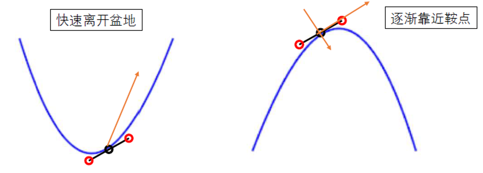
4. Dimer Translation: Uphill Along the Target Direction and Downhill in the Orthogonal Directions

After the rotation has converged, decompose the average force into components parallel and perpendicular to the dimer direction:

$
\mathbf{F}_{\parallel}=(\mathbf{F}\cdot\mathbf{n})\mathbf{n},
$

$
\mathbf{F}{\perp}=\mathbf{F}-\mathbf{F}{\parallel}.
$

When the dimer direction lies along a negative-curvature direction, moving directly along the physical force would send the system downhill and back toward a local minimum. The force component along the dimer direction must therefore be reversed, while the perpendicular downhill component is retained:

$
\mathbf{F}'=\mathbf{F}{\perp}-\mathbf{F}{\parallel}
=\mathbf{F}-2(\mathbf{F}\cdot\mathbf{n})\mathbf{n},
\qquad C<0.
$

This effective force produces uphill motion along the target direction and downhill motion in the orthogonal directions: the midpoint moves toward higher energy along $\mathbf{n}$ while the energy decreases in the perpendicular directions, bringing the midpoint toward the saddle point. If the current direction is still in a positive-curvature region, the parallel force should not be reversed indiscriminately; the precise translation rule depends on the implementation. A common strategy is to apply the reversed force above once negative curvature is detected, while using ordinary force descent or a preconditioned optimization strategy in a positive-curvature region.

The translation step can be written abstractly as

$
\mathbf{R}{k+1}=\mathbf{R}k+\alphak\mathbf{F}'k,
$

where $\alpha_k$ is the step size or the effective step determined by the optimizer. VASP-VTST can use LBFGS, conjugate-gradient, or other optimizers to translate the midpoint. After translation, the dimer is reconstructed or updated, and the rotation step is repeated so that the local minimum-curvature direction is continuously refined.

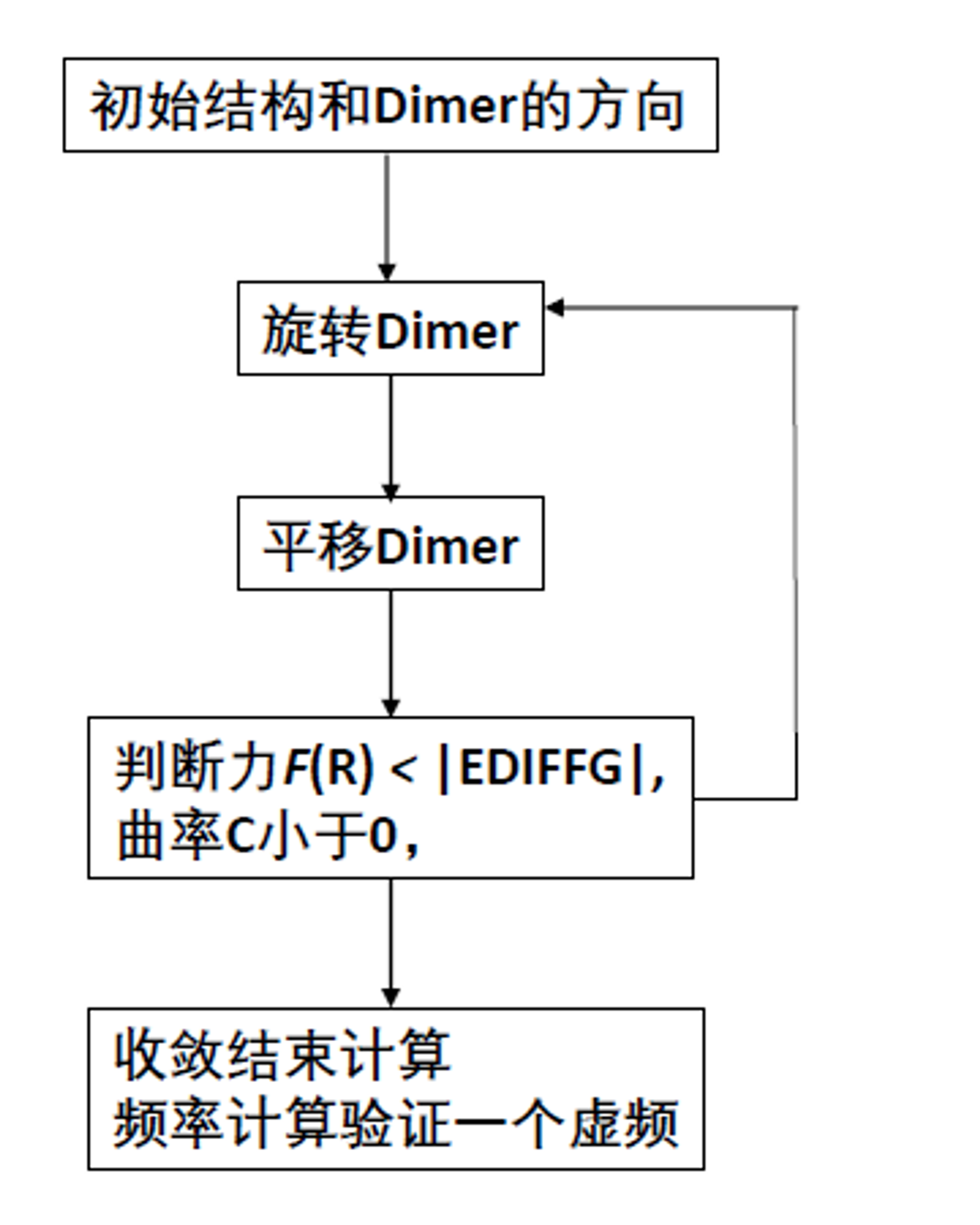
5. Dimer Transition-State Search Workflow

1. Initial setup: Starting from a known configuration $\mathbf{R}$, apply a small perturbation along a selected direction to construct $\mathbf{R}+$ and $\mathbf{R}-$. The initial direction may be chosen from a random displacement, an expected diffusion direction, or a VASP-VTST MODECAR file.
2. Rotate the dimer: Keep the midpoint fixed, calculate the energies and forces at both endpoints, estimate the current directional curvature by finite differences, and iteratively rotate the dimer to find the minimum-curvature direction. This direction is often the gentlest uphill direction toward a nearby saddle point Chemistry Stack Exchange.
3. Translate the midpoint: Once negative curvature is detected, reverse the force component parallel to the minimum-curvature direction so that the midpoint moves uphill along that direction, while retaining the downhill force in the perpendicular directions. This produces the saddle-search force Q-Chem manual.
4. Update the dimer: After each translation, update the midpoint and endpoint positions, then repeat the rotation and curvature evaluation. Because the potential-energy surface changes as the system moves, the dimer direction must be continuously updated.
5. Check convergence: The search is considered close to a first-order saddle point when the maximum midpoint force is below the chosen threshold, the rotational torque is sufficiently small, and the dimer direction has a stable negative curvature VTST Dimer.
6. Output and validate: Save the converged dimer midpoint as a candidate transition-state structure. Displace it slightly forward and backward along the final dimer direction and relax both structures. If the two displacements descend into two different energy basins, the structure is consistent with a saddle point connecting two distinct states. If both displacements return to the same basin, or the energy decreases only negligibly, the result may be a flat region, an incorrect saddle point, or an insufficiently converged structure. When a complete reaction path and a reliable barrier are required, the Dimer candidate can be used to help define the NEB path or endpoints and then be verified with NEB.

DIMER transition-state search flowchart:
The dimer direction corresponds to the minimum-curvature direction in the local quadratic approximation. Near a transition state, this direction generally becomes the imaginary-frequency direction. The effective force $\mathbf{F}'$ drives the system uphill along this direction while allowing downhill relaxation in all other directions, ultimately moving the midpoint toward the saddle point.

6. Common Problems and Computational Considerations

• Dependence on the initial direction: The Dimer method is sensitive to the initial perturbation direction. Different initial directions may converge to different saddle points or may converge slowly. Multiple independent searches with different random directions or MODECAR files are therefore recommended VTST Dimer.
• Validation of a true saddle point: Negative curvature and a small force alone do not prove that the desired transition state has been found. The downhill paths on both sides of the final dimer direction must be checked, and they should lead to two different structures or energy basins.
• Numerical precision: If $\Delta R$ is too small, the force difference amplifies numerical noise; if it is too large, the finite difference no longer represents the local curvature accurately. The dimer separation, EDIFF, force-convergence threshold, and energy cutoff should therefore be tested together. A persistently large torque often indicates unsuitable rotation steps, finite-difference steps, or electronic convergence.

.

0.3 VASP-VTST Toolkit

VASP-VTST (Transition State Tools for VASP) provides tools for implementing NEB and Dimer calculations:
http://theory.cm.utexas.edu/vtsttools/scripts.html

• A collection of Perl scripts for preparing input files and analyzing results.
• Modifications to the VASP source code that implement these transition-state search algorithms.

Important scripts include:

• nebmake.pl: Generate initial configurations for an NEB calculation.
• nebef.pl: Monitor NEB convergence.
• nebbarrier.pl: Generate data for the energy-profile plot.
• nebresults.pl: Summarize NEB results.
• modemake.pl: Generate the initial mode for a Dimer calculation.

0.4 NEB Calculation Workflow

0.4.1 Initial- and Final-State Optimization

1. Build the configurations: Place the four required VASP files (INCAR, POSCAR, KPOINTS, and POTCAR) in each directory. The two POSCAR files should represent the unoptimized initial and final states. All files other than POSCAR should be identical in the two directories.
2. Optimize the reactant (initial-state) and product (final-state) structures separately.
3. Use identical calculation parameters (INCAR, KPOINTS, and POTCAR).
4. Ensure that the atom ordering is exactly the same in both POSCAR files. Each row must refer to the same atom in both structures. If some atoms are fixed—for example, the bottom one or two layers in a surface calculation—their positions should preferably be identical in the two POSCAR files.

0.4.2 Generate Intermediate Images and the Initial Path

1. Use dist.pl to check the structural difference between the initial and final states. The script calculates the square root of the sum of squared displacements of corresponding atoms:

   dist.pl initial/CONTCAR final/CONTCAR

A returned value below approximately 5 Å is usually acceptable. Use an odd number of intermediate images to avoid a plateau.

1. Use nebmake.pl to generate the intermediate images:

   nebmake.pl initial/CONTCAR final/CONTCAR N

Here, N is the number of intermediate images and is typically estimated as dist.pl output / 0.8.

The final N specifies the number of inserted images. The script uses linear interpolation; see the VTST script documentation linked above for details. For example, setting N=3 creates directories 00, 01, 02, 03, and 04. Directory 00 contains the initial state from ini/CONTCAR, directory 04 contains the final state from fin/CONTCAR, and directories 01–03 contain the interpolated images. Copy the corresponding initial- and final-state OUTCAR files into the appropriate directories for later analysis.

1. Check whether the generated images are reasonable:

   nebmovie.pl 0

The argument 0 generates an XYZ file from POSCAR; use 1 to generate it from CONTCAR. An .xyz file will be added to each directory. Inspect these files with Jmol or VESTA.

The downloaded nebmovie.pl script does not directly generate movie.xyz when no argument or argument 0 is supplied. If you want the script to generate movie.xyz automatically instead of manually merging the XYZ files from the individual directories, modify nebmovie.pl by commenting out or deleting the second-to-last if statement.

You can also inspect the POSCAR in directory 01 directly with VESTA.

You can additionally use `nebavoid.pl` with argument 1 to ensure that the distance between every pair of atoms in the interpolated images is greater than 1 Å. The argument specifies the minimum allowed distance and may be a decimal value.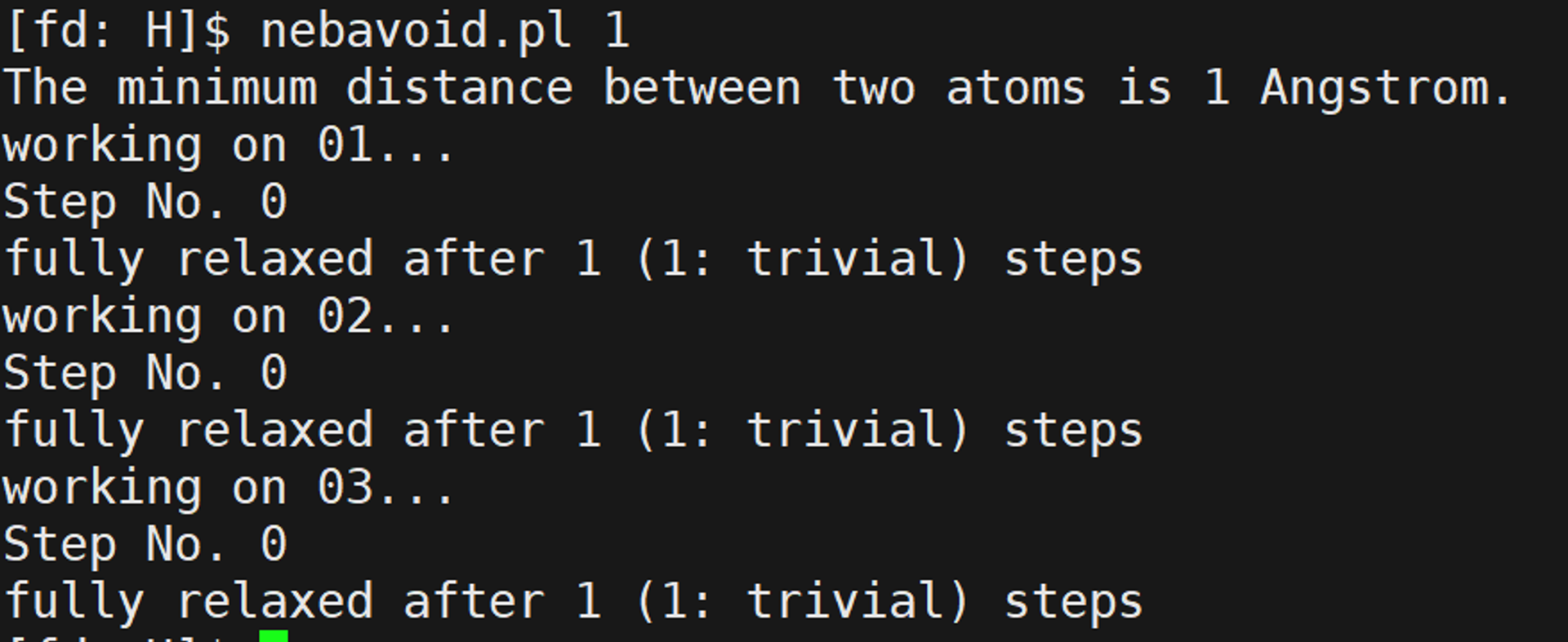

The output above indicates that no interatomic distance is smaller than 1 Å.

An excessively short interatomic distance indicates a structural problem. Either the atoms in the initial and final POSCAR files are not matched correctly, or the linear interpolation used by nebmake.pl is not suitable for estimating the reaction path. In the first case, correct the atom ordering by exchanging the corresponding rows in the CONTCAR files. In the second case, adjust the structures manually with software such as Materials Studio and place the corrected structures in the appropriate directories.

0.4.3 Prepare the NEB Calculation Files

1. Set up the INCAR file:

   ICHAIN = 0         # Enable NEB
   LCLIMB = .TRUE.    # Use CI-NEB
   IOPT = 1           # VTST optimizer
   IMAGES = N         # Number of intermediate images
   SPRING = -5        # Spring-force constant
   IBRION = 3
   POTIM = 0
   EDIFF = 1E-7       # Tight electronic convergence
   EDIFFG = -0.03     # Ionic convergence criterion

To use a VTST optimizer, set IBRION=3 and POTIM=0 as shown above; choose IOPT according to the optimizer recommendations. If you use a VASP-native optimizer, use IBRION=1 or 3, not 2, and test an appropriate POTIM in the range 0.01–0.5.
A transition-state calculation is also a structural optimization. Start from the structural-optimization `INCAR` and modify it as follows:

• EDIFF=1E-7: This parameter is particularly important. Transition-state calculations require highly accurate forces; tighter electronic convergence produces more accurate forces and can accelerate convergence. Many failed transition-state calculations are caused by insufficient force accuracy. For a preliminary calculation, this can be relaxed to 1E-5.
• EDIFFG=-0.03: The structural convergence criterion can generally be relaxed to -0.03 for a transition state, or to -0.05 for especially difficult systems.
• IBRION=3, POTIM=0: These settings tell VTST to activate its optimizer.
• IOPT=1: Select the optimizer according to the recommendations. IOPT=7, 2, or 1 are commonly recommended. IOPT=0 activates the VASP-native optimizer; for example, IOPT=0 with IBRION=1 and POTIM=0.1.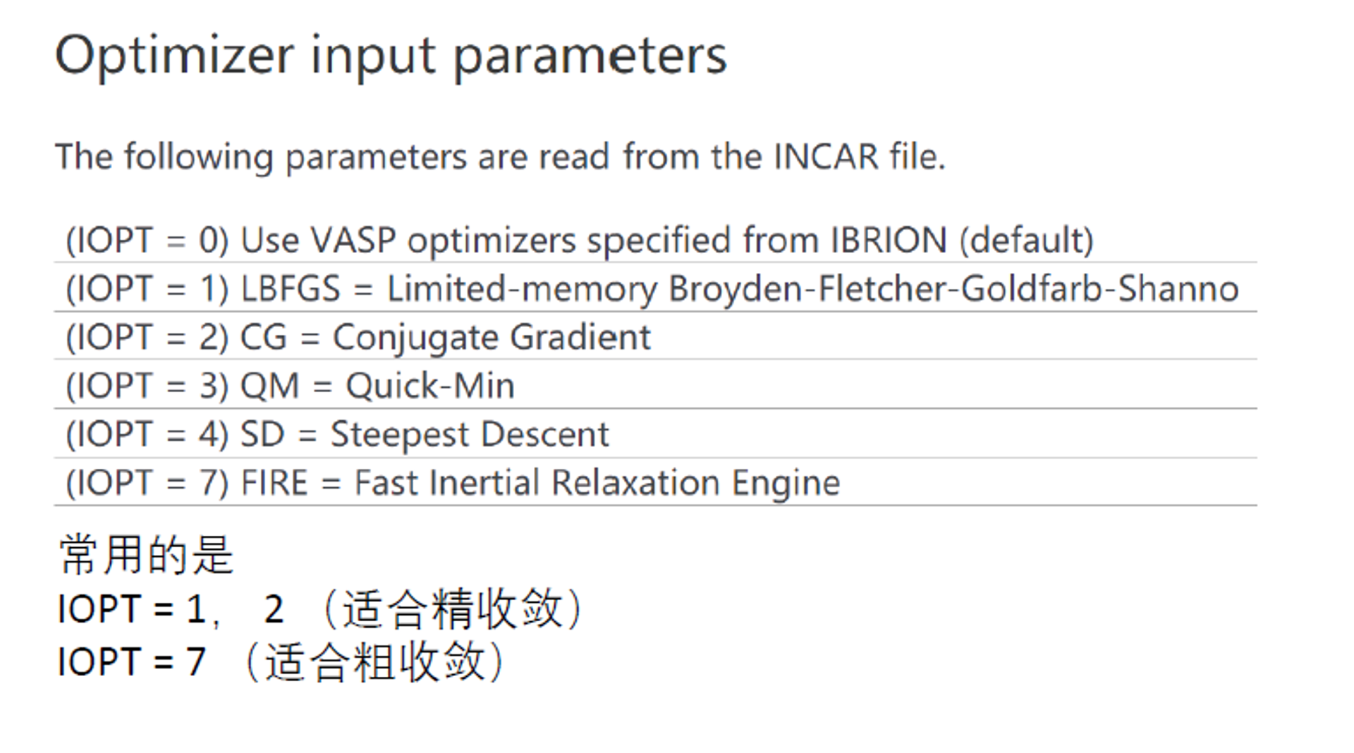
• 
• ICHAIN=0: Enable the NEB algorithm.
• LCLIMB=.TRUE.: Enable climbing-image NEB.
• IMAGES=1: Specify the number of intermediate images.
• SPRING=-5: Use -5 as the spring-force constant.

1. Prepare the KPOINTS and POTCAR files using the same settings as in the structural optimization.

0.4.4 Submit and Monitor the Calculation

1. Use a VASP executable compiled with VTST.
2. The number of CPU cores should be divisible by the number of images.
3. Monitor convergence with nebef.pl or nebefs.pl:

   nebef.pl

In the output, the second column is the maximum force (force of images in the neb), and the third column is the energy of the corresponding structure.

In the INCAR settings above, EDIFFG=-0.02 means that the calculation terminates when the maximum force on every structure is below 0.02 eV/Å. A value of -0.02 is common for ordinary structural optimization, while -0.03 is often used for NEB calculations. The calculation is converged only when the maximum atomic force on every intermediate image is smaller than |EDIFFG|.

Another command for monitoring convergence is `nebbarrier.pl`. It takes no argument, does not print results to the screen, and instead generates a neb.dat file.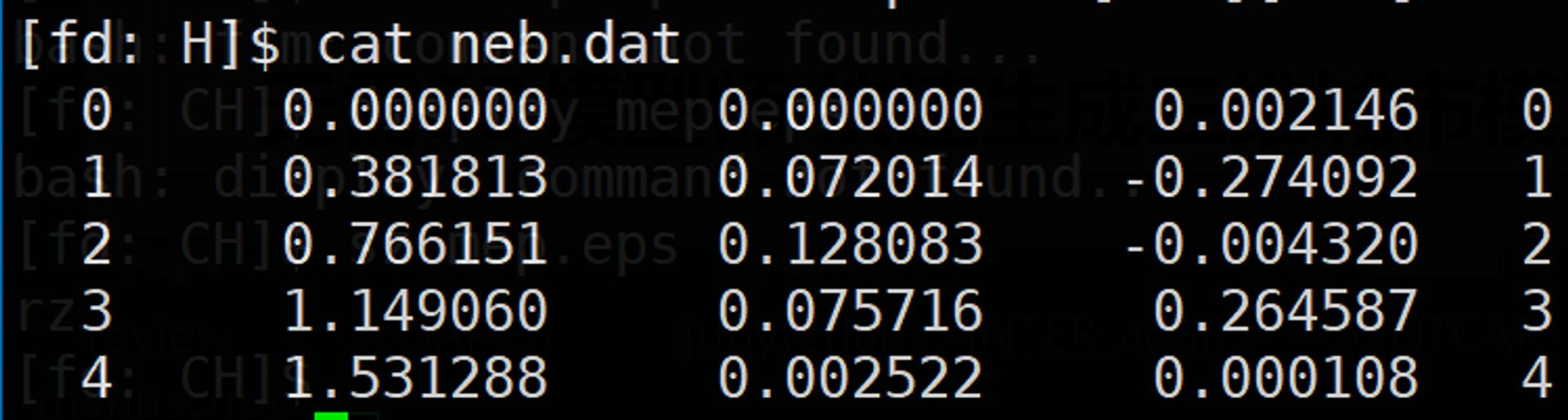

In neb.dat, the second column is the distance, corresponding to the dist.pl result between neighboring structures; the third column is the energy relative to the initial state; and the fourth column is the force along the NEB path.

The force associated with EDIFFG is the force of images in the neb reported by nebef.pl.

0.4.5 Analyze the Results

1. Summarize the results with nebresults.pl:

   nebresults.pl

As indicated by its output, nebresults.pl runs nebbarrier.pl, nebspline.pl, nebef.pl, nebmovie.pl, nebjmovie.pl, and nebconverge.pl, and packages the OUTCAR files from the individual directories. It generates many files. Among them, mep.eps is an energy-barrier plot with the dist.pl distance on the horizontal axis and energy on the vertical axis.

1. Analyze the mep.eps energy profile.


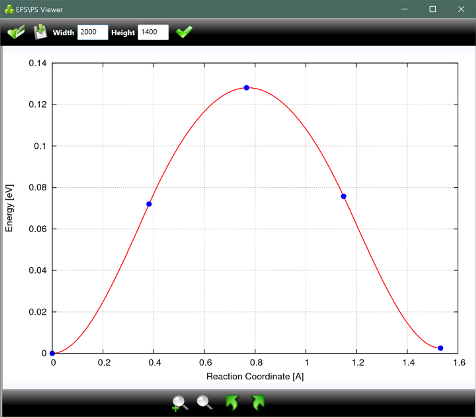
This file may not open in ordinary image viewers; EPS/PS Viewer is recommended. Download EPS Viewer
The generated spline.dat file contains the fitted curve data for the points above. Once the plotted curve is available, these raw data are usually less important.

1. Check the convergence plots in the vaspgr directory.

The vaspgr directory contains convergence plots for each interpolated image. They can also be opened with EPS/PS Viewer; for example, vaspout1.eps contains the convergence information for image 01.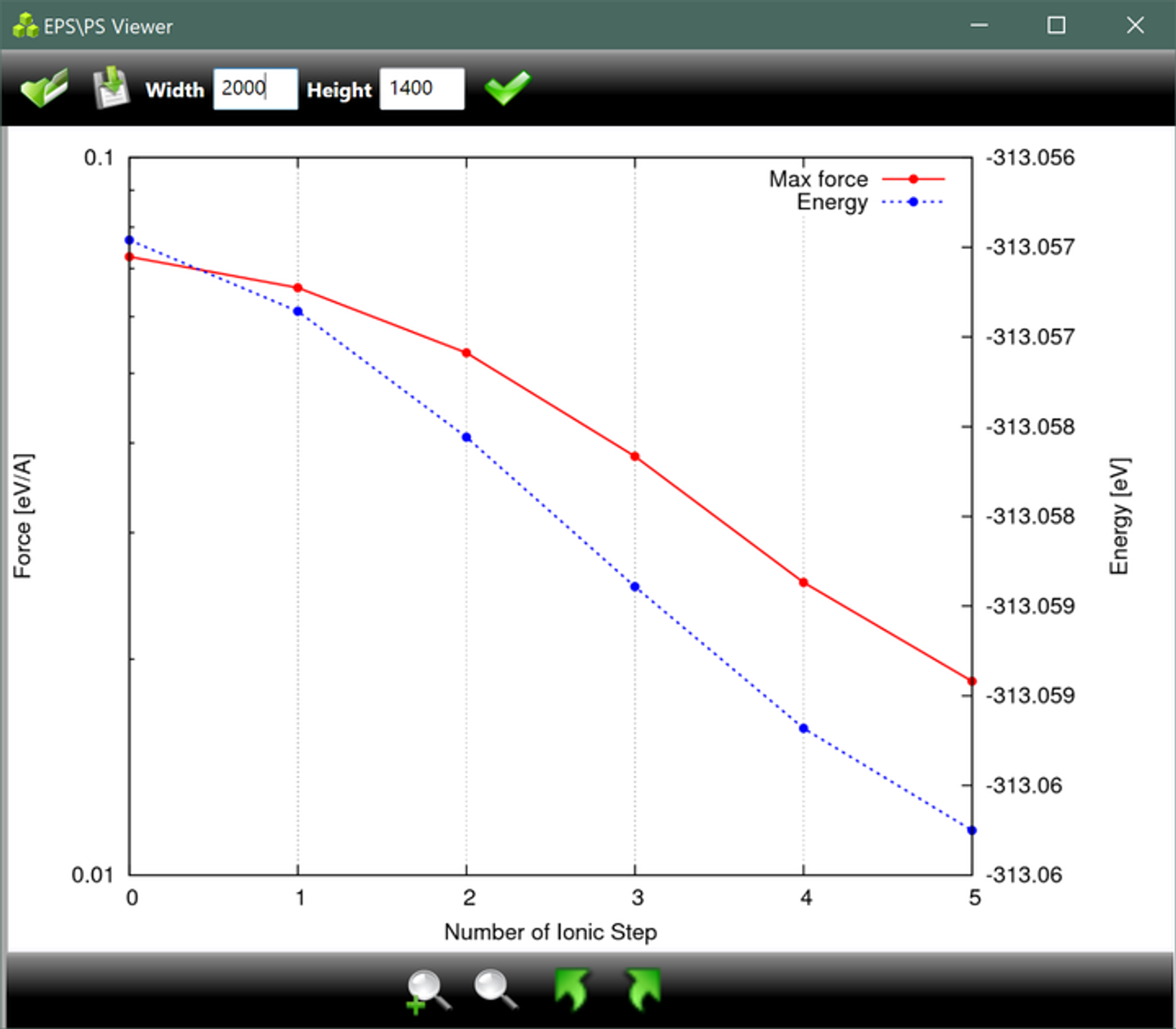


2. Verify the transition state with a frequency calculation. A first-order saddle point should have exactly one imaginary frequency.

0.5 DIMER Calculation Workflow

0.5.1 Prepare the Initial Structure

A Dimer transition-state calculation does not require the initial state (IS) and final state (FS), but these states will eventually need to be calculated. Optimizing the initial and final states before the transition-state search helps to construct a good initial guess and provides a general understanding of the reaction process.

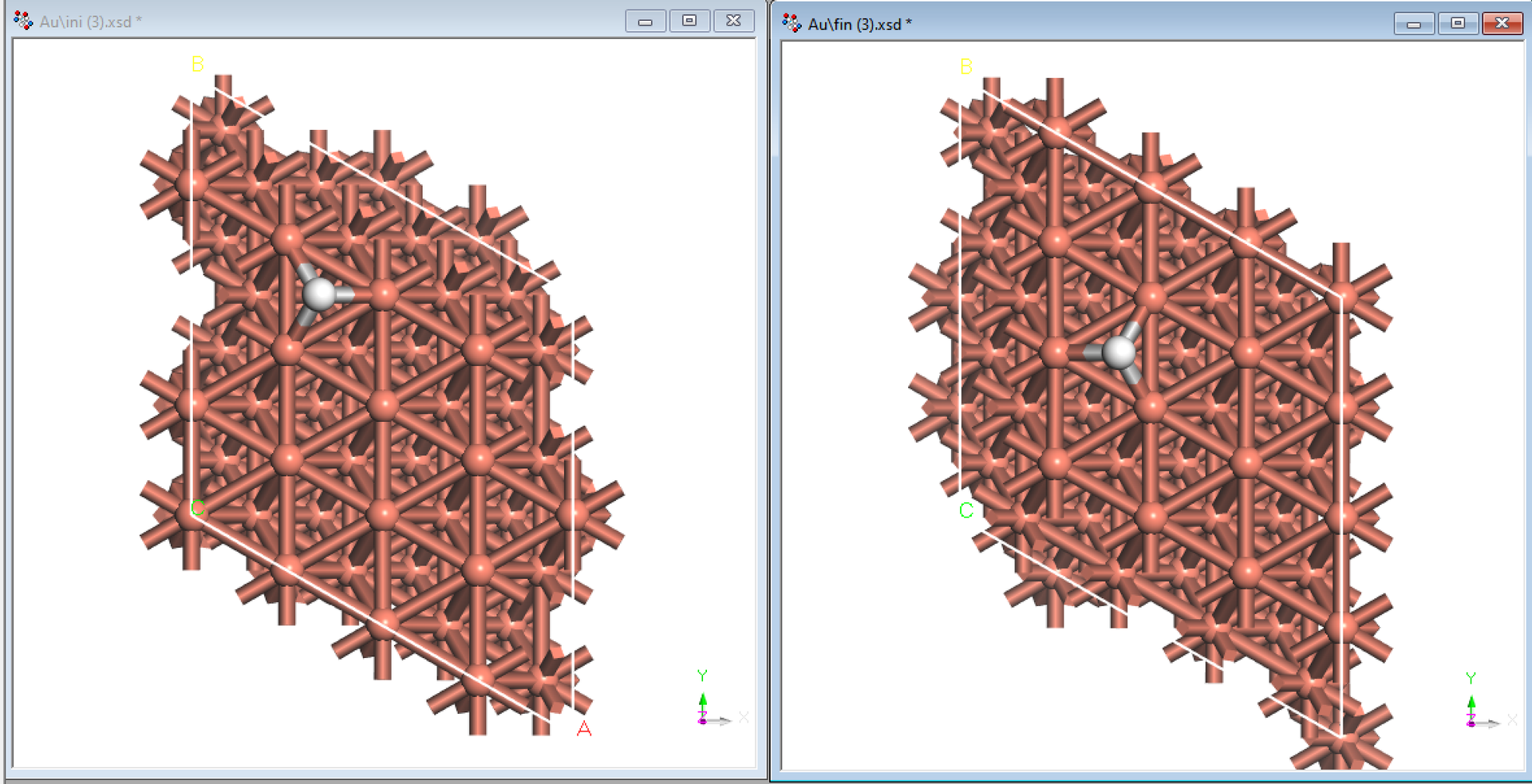
The initial guess can be prepared by manually modifying the initial or final state in Materials Studio. Download the initial-state CONTCAR, convert it to CIF format, import it into Materials Studio, and manually adjust it toward a plausible transition-state structure. Save the CIF file and convert it back to POSCAR. Alternatively, use nebmake.pl to generate several intermediate images and select one as the initial Dimer structure.

Constructing a good initial guess is often the most technically demanding part of a transition-state search. Its quality strongly affects both the probability of convergence and the computational time. The initial structure should be as close as possible to the transition state, which generally requires experience with the system. One basic rule is to avoid excessively short bonds. Very short bonds create strong repulsion, which can cause the structure to collapse during the first few ionic steps and move away from the transition state. For example, in O diffusion, if the O atom crosses the barrier at constant $z$ coordinate, the Au–O bond at the bridge transition site may be shorter than the Au–O bond at the hollow site. The O atom should therefore be slightly higher in the $z$ direction at the transition state.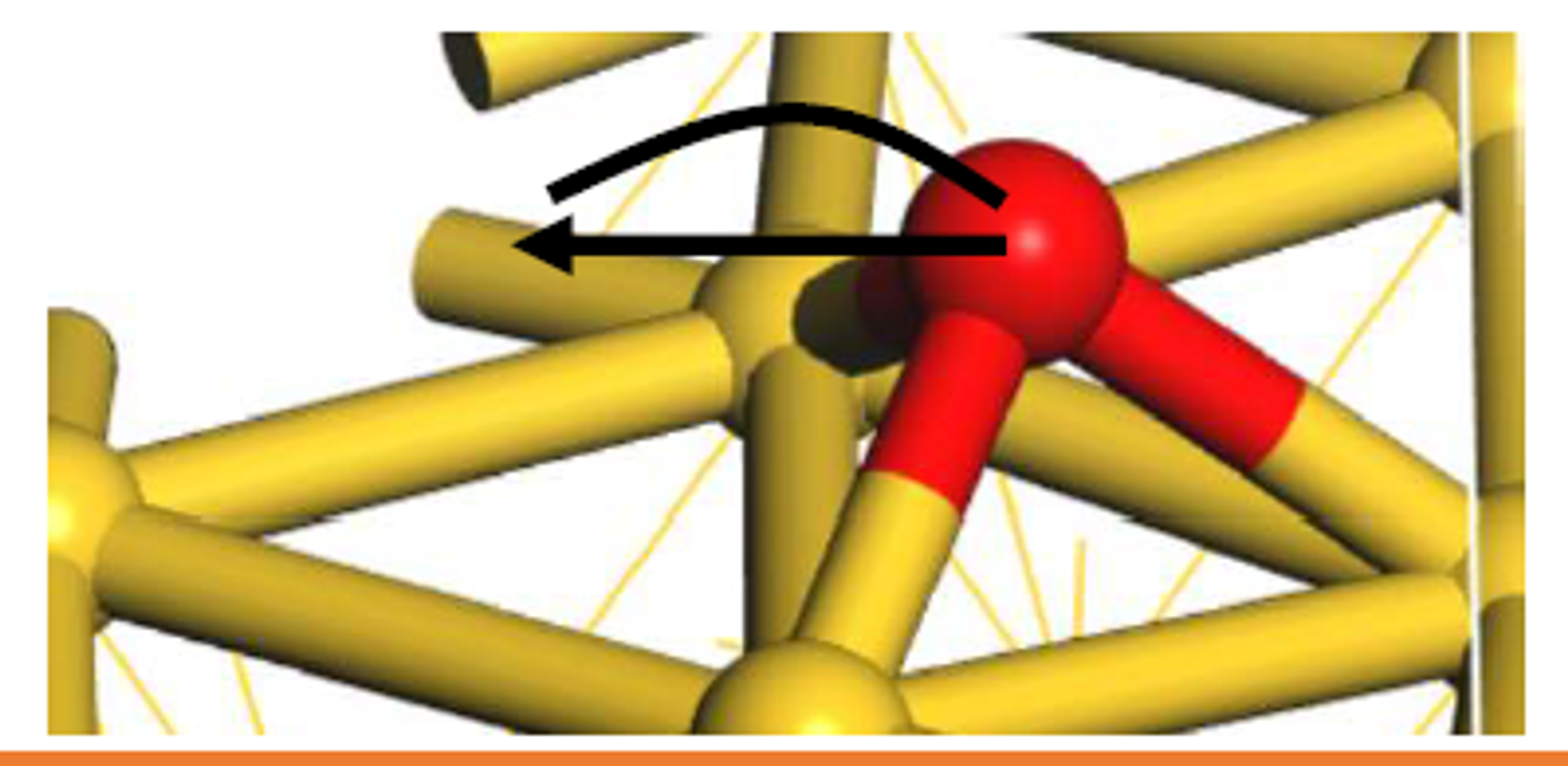

0.5.2 Generate the MODECAR File

The calculation additionally requires a MODECAR file defining the initial dimer direction. If this file is absent, the program generates a random initial direction; setting MODECAR explicitly is strongly recommended.

The VTST script modemake.pl generates MODECAR by subtracting the initial-state coordinates from either the guessed transition-state coordinates or the final-state coordinates, followed by normalization. The resulting file represents a displacement vector.

Use modemake.pl as follows:

modemake.pl initial/CONTCAR final/CONTCAR

or

modemake.pl initial/CONTCAR ./POSCAR

For the second command, delete the atomic-velocity section at the end of is/CONTCAR so that it has the same number of lines as POSCAR.

0.5.3 Introduction to MODECAR

MODECAR defines the dimer direction, which is also the expected imaginary-frequency mode. Once the Dimer calculation starts, NEWMODECAR is updated after each dimer-rotation step with the current dimer direction.

-7.1542374114E-15 7.7446891786E-15 2.0281291017E-14
0.0000000000E+00 0.0000000000E+00 -6.0531853189E-14
1.3589288129E-05 2.2051181757E-05 3.2922406528E-05
-1.7569180080E-05 2.1509134997E-05 -3.5180020535E-05
-2.9870725746E-05 1.6276168673E-06 2.5483359881E-05
。。。
。。。
-1.3414195146E-14 7.7446891786E-15 2.0281291017E-14
0.0000000000E+00 0.0000000000E+00 -6.0531853189E-14
-1.6898717065E-05 8.9460297249E-06 3.0936372624E-05
-4.6190423810E-06 1.2930524264E-05 4.5824912007E-05
1.2817823937E-05 9.1025990586E-06 7.1181188675E-05
2.4199310346E-01 9.3308559935E-01 1.6190951779E-01

0.5.4 Prepare the DIMER Calculation Files

Key INCAR settings:
Start from the structural-optimization INCAR and modify it as follows: (1) ICHAIN=2 enables the Dimer algorithm in VTST. (2) IBRION=3, POTIM=0 tell VTST to activate its optimizer. (3) Set IOPT=2 according to the optimizer recommendations. For stable transition-state convergence, IOPT=7, 2, or 1 are commonly recommended. IOPT=0 activates the VASP-native optimizer; for example, IOPT=0 gives IBRION=1 and POTIM=0.1. (4) EDIFF=1E-7 is particularly important. Because the two dimer endpoints are very close, the forces must be highly accurate. Tighter electronic convergence produces more accurate forces and can accelerate convergence; many failed transition-state calculations are caused by insufficient force accuracy.
(5) EDIFFG=-0.03: The structural convergence criterion can generally be relaxed to -0.03 for a transition state, or to -0.05 for especially difficult systems.

ICHAIN = 2      # Enable Dimer
IOPT = 2        # VTST optimizer
IBRION = 3
POTIM = 0
EDIFF = 1E-7
EDIFFG = -0.03

0.5.5 Submit and Monitor the Calculation

1. Use a VASP executable compiled with VTST.
2. Monitor the changes in Force, Torque, and Curvature in DIMCAR.

Transition-state calculations are more difficult to converge than ordinary structural optimizations, so allow sufficient time. Monitor convergence during the run. If the structure deviates severely from the expected transition-state configuration, terminate the job and revise the initial structure.

During a Dimer calculation, VTST outputs several useful files: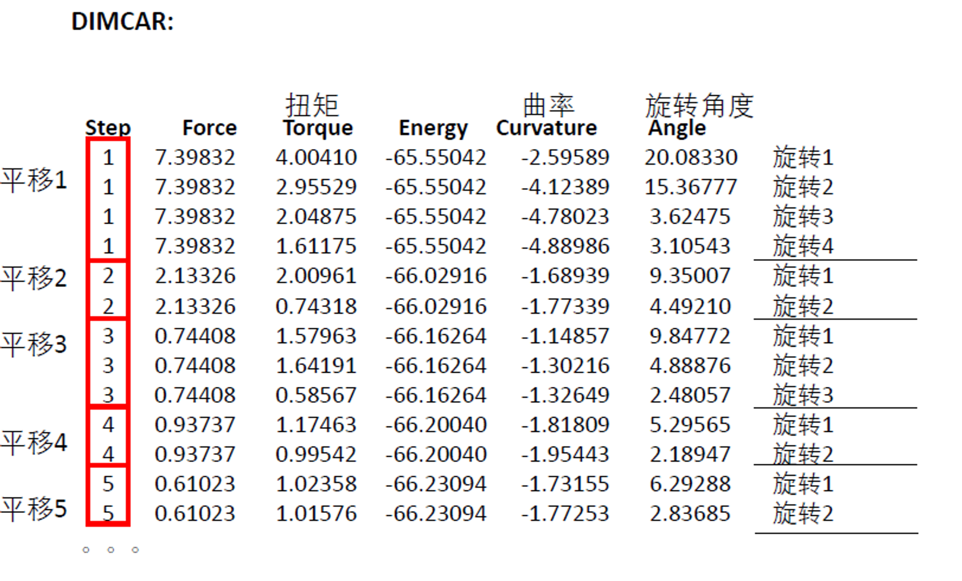

DIMER output:

• step: The number of dimer-translation steps. Each translation step may contain several dimer-rotation steps.
• Force: The maximum force over all degrees of freedom of the dimer. Force < |EDIFFG| is not by itself the convergence criterion. The actual criterion is that the maximum atomic force satisfies $F < |EDIFFG|$; inspect it with grep RMS OUTCAR.
• Torque: The dimer torque. During rotation, the Dimer moves in the direction that reduces the torque. When Torque < 1, the calculation proceeds to a dimer-translation step.
• Energy: The energy of the dimer midpoint. This is not the energy extrapolated to zero electronic entropy, so it should not be used as the final transition-state energy. Use the final E0 value in OSZICAR for that purpose.
• Curvature: The dimer curvature. Rotation turns the dimer toward the minimum-curvature direction, and the curvature should generally decrease during each translation step. At the transition state, the dimer direction corresponds to the reaction direction.
• Angle: The dimer rotation angle. The angle should generally decrease during each translation step.

The most important quantities are Force, Torque, and Curvature. During dimer rotation, Torque should continuously decrease. If it does not, improve the force accuracy by using a tighter EDIFF, PREC=Accurate, or a larger DdR such as DdR=0.01. A gradual decrease in Force together with negative Curvature indicates approach to the transition state. If the curvature is not negative, the system is probably still far from the transition state and the calculation should continue.

0.5.6 CENTCAR and NEWMODECAR Files

During a Dimer calculation, the direction and position are continuously updated. After each dimer-translation step, the midpoint position and the latest dimer direction are written to CENTCAR and NEWMODECAR. CENTCAR has the same format as POSCAR and CONTCAR, while NEWMODECAR has the same format as MODECAR.

Use dimmode.pl to generate dimmode.xyz for visualizing the vibrational direction.

dimmode.pl CENTCAR NEWMODECAR 32 0.5 (default)
dimmode.pl CENTCAR NEWMODECAR 16 1 (recommended)

Note that the first line of CENTCAR must contain the element symbols.

The script creates an animation centered at CENTCAR and oriented along the vibrational direction in NEWMODECAR. The resulting dimmode.xyz file can be opened with Jmol, VMD, or similar programs. In Jmol, use Tools → Animate → Loop.

0.5.7 Analyze the Results

The command

grep converged OUTCAR

should return the field OPT: skip step - force has converged.

In this example, the calculation required 207 ionic steps and 9,620 seconds. We set EDIFFG=-0.01, but the Force in DIMCAR converged before reaching 0.01; this is normal. To inspect the maximum atomic force, use:

grep RMS OUTCAR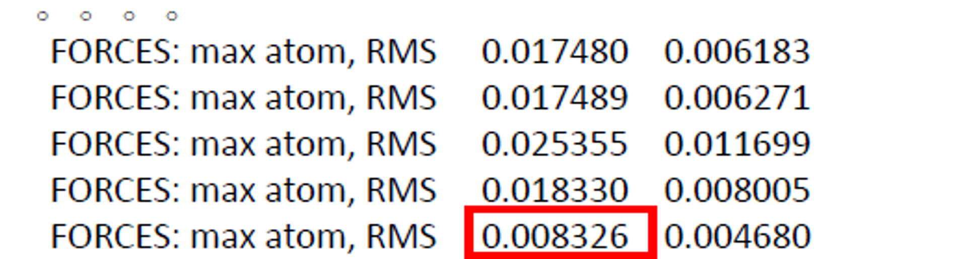

The final force is smaller than |EDIFFG|, so the transition-state calculation has converged normally. Use tail -1 OSZICAR and take the final E0 value as the transition-state energy:

F= -.66261570E+02 E0= -.66258695E+02 d E =-.705902E-05

0.6 Other Methods

Methods for locating transition states in VASP include:

• Methods based on a single initial guess (Dimer).
• Methods based on both reactant and product structures (CI-NEB).
• Methods based on the reactant structure (SSW).
• Potential-energy-surface scanning.

For a detailed introduction, see:
http://sobereva.com/44

0.7 Common Problems and Solutions

1. An intermediate image in the CI-NEB calculation has lower energy than both the initial and final states.

Solution: There are two possible explanations. First, at least one additional local minimum may exist between the initial and final states. Second, the initial and final states may not themselves be fully optimized minima. Recalculate them using tighter settings.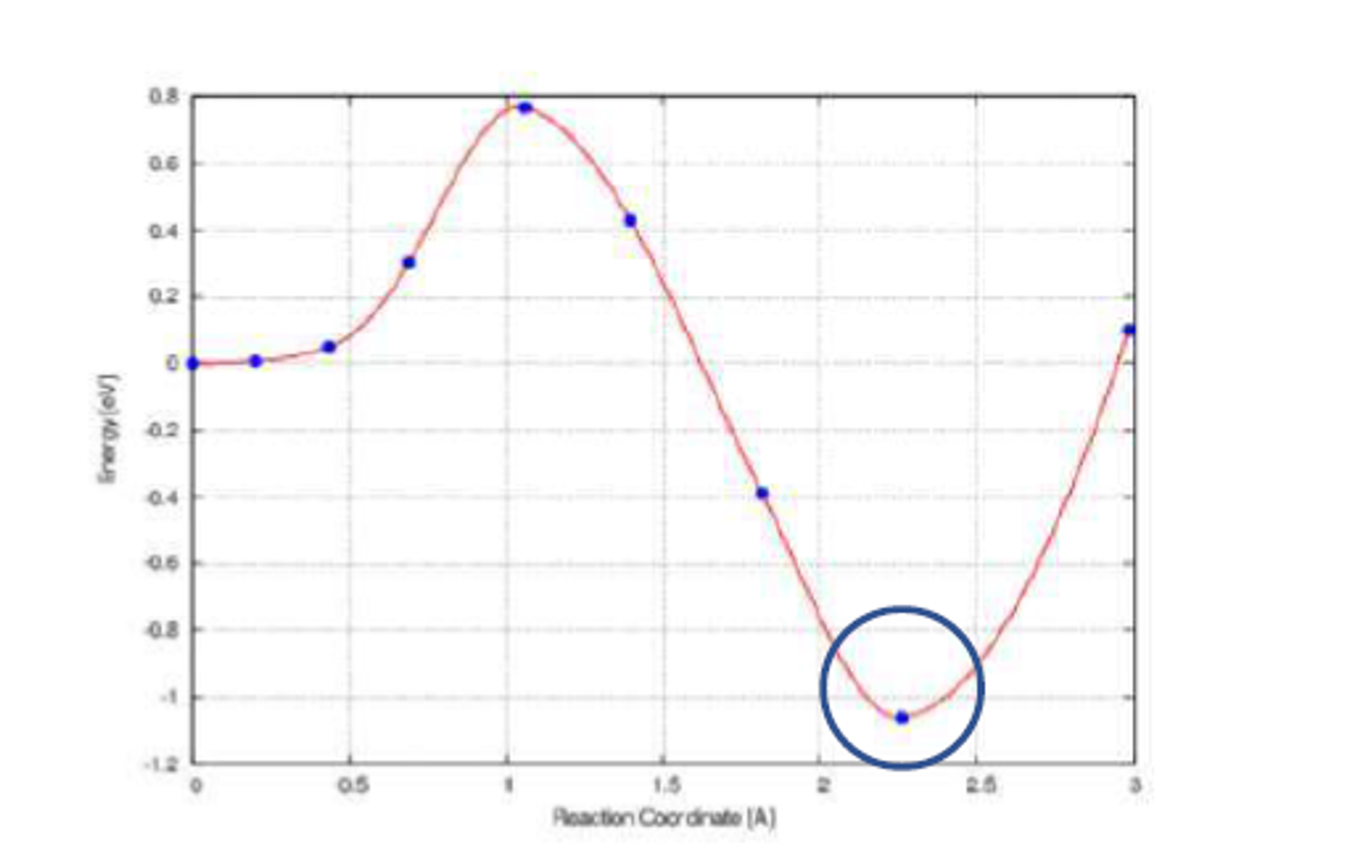


2. 2. Extremely large atomic forces appear at the beginning of the CI-NEB calculation, for example above 10 eV/Å.

Solution: The initial path is almost certainly unreasonable. Use nonlinear interpolation, such as the `idpp.py` script, or download the problematic POSCAR and adjust the structure manually.

1. 3. The calculation is close to convergence, but the forces remain above the convergence threshold for a long time.

Solution: There are several possible causes. The force accuracy may be insufficient; try PREC=Accurate and EDIFF=1E-7. The transition-state optimizer may also be unsuitable; try IOPT=7 or IOPT=0 with the VASP-native DIIS optimizer. The force-convergence threshold may also be too strict.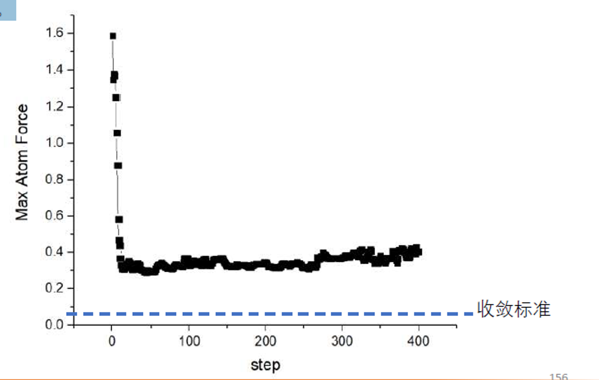


2. The transition-state calculation converges, but the frequency calculation shows no imaginary frequency or more than one imaginary frequency.

Solution: If there is no imaginary frequency, the result is not a valid first-order saddle point; insufficient force accuracy is the most likely cause. Multiple imaginary frequencies may also result from insufficient force accuracy. Use a strict EDIFF=1E-7 or switch to the Dimer method. Very small imaginary frequencies may be neglected, especially when they correspond to translational modes.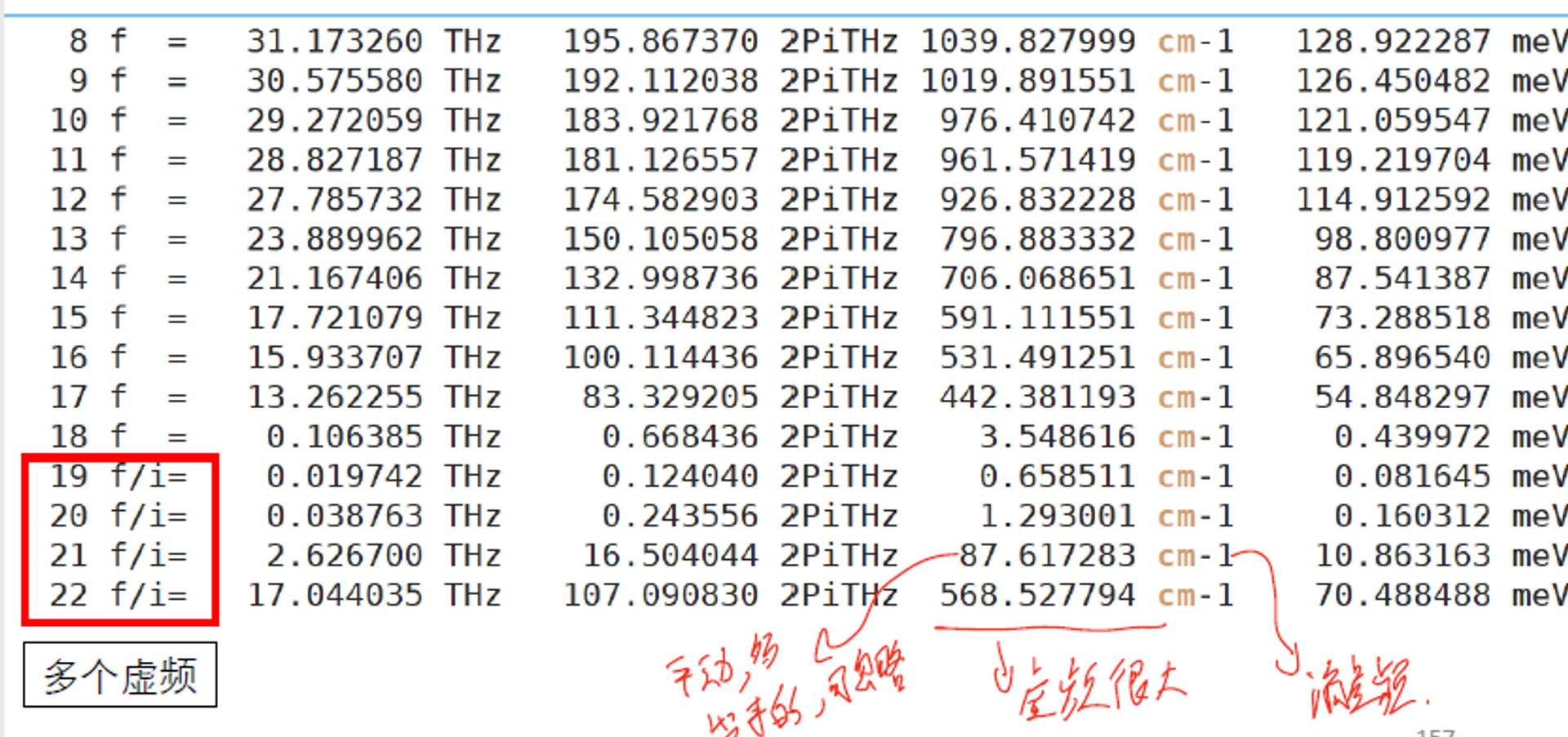


3. 5. If the structures generated by nebmake.pl are highly disordered, check the initial and final

state atom ordering. Each atom must correspond exactly between the two structures. This is a common beginner error, so preserve the same atom ordering when preparing both states.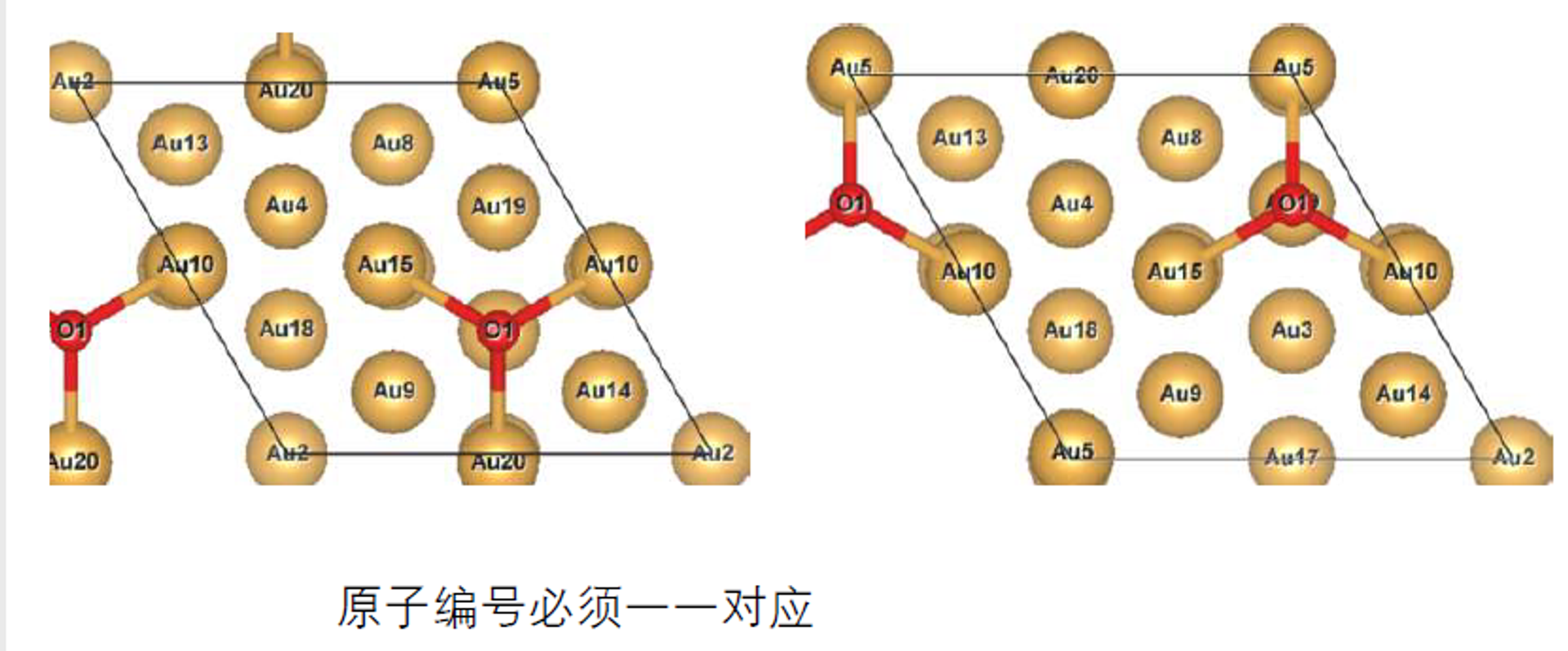

1. One image has a very large force.

• Check whether the initial path is reasonable. Ensure that the initial and final states are fully optimized and that the path interpolation is sensible.
• Increase the magnitude of SPRING while keeping it negative to strengthen the elastic force between images.
• Initially disable the climbing image and enable LCLIMB=.TRUE. only after the path has approximately converged.
• Check whether a special structural change or energy barrier exists near the image with the large force. More images may be needed in that region.
• Use an optimizer from the VTST toolkit, such as FIRE or BFGS. These optimizers may be more effective for NEB calculations.
• If the problem persists, manually adjust the structure of the problematic image and restart the calculation.
• For a complex system, first perform a preliminary convergence using lower-accuracy settings, then repeat the calculation with high-accuracy parameters.

1. Techniques for accelerating convergence

• In terms of the IOPT=3 settings, the primary control is with the TIMESTEP variable. If the value is too small, convergence will be slow. The rate of convergence will increase as the TIMESTEP value is increased until the method becomes unstable. A value of 0.1 is generally safe, but the actual value will depend upon the stiffest vibrational frequencies in your system. The MAXMOVE value can be safely set to something like 0.1 - 0.5 Ang and left alone - it is really just a sanity parameter to make sure that no optimizer moves the system more than a sensible trust-radius.
• Simplified calculation settings: Consider using softer pseudopotentials, such as O_s instead of O and Zr instead of Zr_sv, reduce ENCUT to approximately 240 eV, and use Gamma-point sampling to accelerate the calculation.
• Switch to the Dimer method: Starting from a moderately converged NEB calculation, use the Dimer method to locate the saddle point more precisely. This may further improve convergence.
• Restart and refinement strategy: First locate the geometry quickly using lower-accuracy settings, then gradually increase the accuracy and reconverge to assess the sensitivity of the result to each parameter.
• Adjust POTIM as needed. If POTIM is too small, the configuration of CH₄ in the initial images may change insufficiently, which can impair overall convergence. This advice applies to the NEB method.

0.9 Plot an Ionic-Diffusion Path

To plot an ionic-diffusion path, you only need VESTA and the `POSCAR` files generated after image interpolation.

After interpolation with NEB, several directories containing intermediate POSCAR files are generated. Import these POSCAR files into VESTA in sequence to visualize the approximate diffusion path. For example, if Li atom 7 is removed from the initial structure and neighboring Li atom 8 gradually moves into the original position of atom 7, the final structure has no Li at the original position of atom 8 and has Li at the original position of atom 7.

To plot the diffusion path, manually combine the relevant coordinates from all intermediate POSCAR files into one POSCAR. Do not concatenate the complete files with `cat`; copy only the `x`, `y`, and `z` coordinates of the migrating atom into a new `POSCAR`.

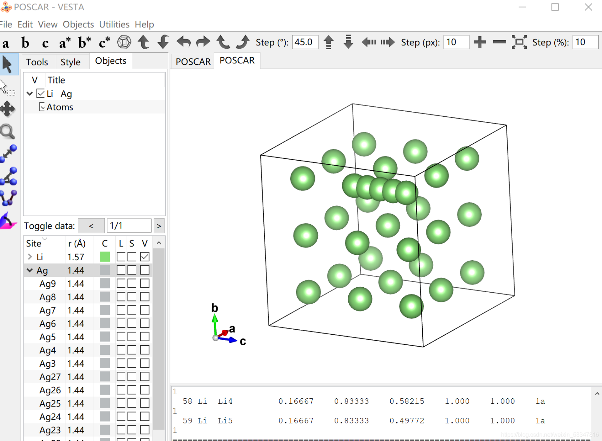
Detailed procedure: Open the original POSCAR containing the complete unit cell. Add the name and number of the migrating atom on lines 6 and 7, respectively, and then append the migrating-atom coordinates after the existing coordinate list. For example, for Li diffusion in LiAg, suppose atom 8 migrates to the original position of atom 7. The moving atom is therefore atom 8, and the five directories 00–04 generated by interpolation represent its path. Open the original complete-cell POSCAR, add Li on line 6 and 5 on line 7, then open the POSCAR in each directory from 00 through 04, locate the one-line x y z coordinates of atom 8, and append those coordinates to the original POSCAR.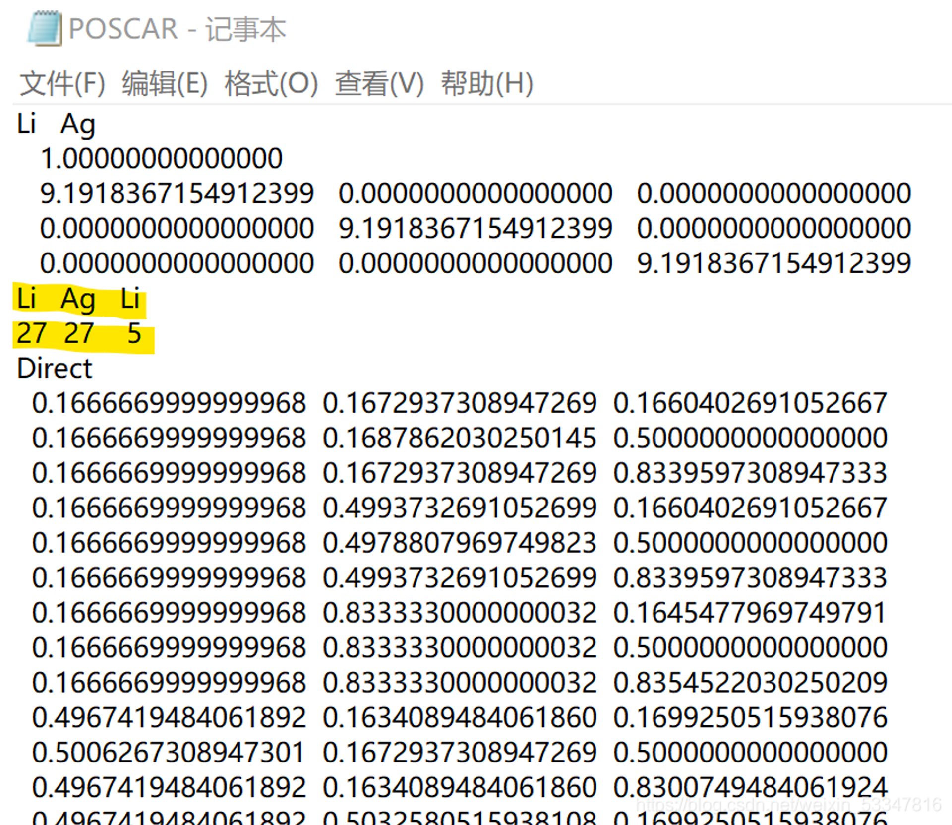

Official VTST Documentation

[Nudged Elastic Band] Options

Variable	Default Value	Type	Description
ICHAIN	0	int
IMAGES	none	int	Number of NEB images between the fixed endpoints
SPRING	-5.0	float	The spring constant, in eV/Ang^2 between the images; negative value turns on nudging
LCLIMB	. TRUE.	boolean	Flag to turn on the climbing image algorithm
LTANGENTOLD	. FALSE.	boolean	Flag to turn on the old central difference tangent
LDNEB	. FALSE.	boolean	Flag to turn on modified double nudging
LNEBCELL	. FALSE.	boolean	Flag to turn on SS-NEB. Used with ISIF=3 and IOPT=3.
JACOBIAN	(Ω/N)^{1/3}N^{1/2}	real	Controls weight of lattice to atomic motion. Ω is volume and N is the number of atoms.

Several support programs are available for setting up dynamical-matrix calculations in VASP and processing their output. Descriptions of these programs, most of which are Perl scripts, can be found at the following page:

SCRIPTS — Transition State Tools for VASP

Required Parameters

Parameter	Default Value	Description
ICHAIN	1	Use the Dynamical Matrix method
IBRION	3	Specify that VASP do MD with a zero time step
POTIM	0	Zero time step so that VASP does not move the ions
EDIFF	1 E-8	Strict force criteria to accurately find force differences (curvature)
EDIFFG	1 E-8	Make sure that vasp does not quit if the forces are low
NSW	DOF+1	Do a force call at equilibrium and along each degree of freedom

Setting up a dynamical matrix calculation

1. Compile a VASP version using the VTST source code.

1. Select the degrees of freedom to calculate in DISPLACECAR. This file is a list of displacements with dimensions $3\times N$, where $N$ is the number of atoms. A typical displacement in the list is on the order of 0.001. The file can also be generated with dymselsph.pl, which selects atoms within a specified radius of a central atom for molecular vibrational-frequency calculations, or with dymseldsp.pl, which selects atoms with the largest displacement between two POSCAR files.

1. The calculation can run with a single image, calculating one displacement at a time, or with multiple images, calculating several displacements simultaneously. If you use single-image mode, no action is needed at this step. For parallel execution, choose a number of images $M$ that divides the number of displaced degrees of freedom (DOF) evenly. Then create $M$ subdirectories numbered 01 through M, using two digits for each directory name, and place a POSCAR file in each subdirectory.

1. Set up the INCAR file with ICHAIN=1, POTIM=0.0, IMAGES=M (only when running multiple geometries in one calculation), and NSW=(DOF/M)+1. The additional 1 is required because each calculation evaluates the forces of the initial structure before applying any displacement.

For NSW, use one more ionic step than the number of degrees of freedom in a single-image calculation. In a parallel calculation, use one more step than the number of degrees of freedom divided by the number of images $M$. For example, a single-image calculation for ethane has 24 degrees of freedom (3 per atom for 8 atoms), so set NSW=25. If the calculation is parallelized over $M=4$ images, set IMAGES=4 and NSW=(24/4)+1=7.

1. After verifying that POTCAR, POSCAR, INCAR, DISPLACECAR, and KPOINTS are present and correctly configured, run VASP. To ensure accurate modes, first optimize the geometry in POSCAR with VASP. All INCAR settings used in the geometry optimization, such as ISMEAR, SIGMA, and PREC, should also be present in the dynamical-matrix INCAR.

1. Extract the force constants from the output with dymmatrix.pl; consult the script documentation for its arguments. The script outputs the dynamical matrix, its eigenvalues, normal-mode frequencies, and normal-mode eigenvectors. Examples include:

For a single calculation with a single image:

dymmatrix.pl DISPLACECAR OUTCAR

For a single calculation with multiple images:

dymmatrix.pl 1 DISPLACECAR ??/OUTCAR

For multiple calculations with $n$ DISPLACECAR and OUTCAR files:

dymmatrix.pl n DISPLACECAR 1 .. DISPLACECARn OUTCAR 1 .. OUTCARn

1. If all calculated frequencies are zero, check the EDIFFG tag in the dynamical-matrix INCAR. When running the dynamical-matrix code after geometry minimization, this tag can be set to an arbitrarily small value to prevent the calculation from terminating early as though the structure were already converged. The number of force calls should equal the number specified by NSW.

1. Check frequency convergence with respect to all parameters, especially the finite-difference displacement in DISPLCECAR, the force accuracy, and the smearing width. A small smearing width is particularly important when calculating normal modes for molecules with a large HOMO–LUMO gap.

1. Calculate the prefactor; this step is not needed for a simple frequency analysis. The dymprefactor.pl script performs this calculation. It takes the eigenvalue files of the minimum and transition state as input and outputs the prefactor in inverse centimeters.

Calculating additional degrees of freedom

This completes one prefactor calculation. To perform another calculation for the same system while including additional degrees of freedom:

1. Save the OUTCAR file from the previous calculation.
2. Create a new DISPLACECAR following the previous procedure.
3. Use dymcmpdisp.pl to generate the difference between the new and old DISPLACECAR files. Run the dynamical-matrix code using this output.
4. Modify NSW in the INCAR file as before.
5. Run VASP.
6. Extract the forces from the OUTCAR files using dymmatrix.pl. You will need the original calculation's DISPLACECAR, the current calculation's DISPLACECAR, and all corresponding OUTCAR files. Again, the second and subsequent DISPLACECAR files should contain only the new degrees of freedom that were not calculated previously.

FORCE BASED OPTIMIZERS

The NEB and min-mode following (dimer/Lanczos) saddle point finding methods use a force projection in order to direct the optimizers towards minimum energy paths and saddle points. These modifications to the force mean that the energy is no longer consistent with the force being optimized. Because of this, we can only use optimizers that are solely based upon the force (and not the energy). The quasi-Newton and quick-min (IBRION=1 and 3 respectively) optimizers that are built into VASP are both force-based, but the conjugate-gradient method (IBRION=2) is not.

Here, we present a set of optimizers that are all force-based so they can be used with the NEB and min-mode following methods. To use them, the INCAR must set IBRION=3 and POTIM=0, to disable the built in optimizers. Then, the IOPT parameter will select one of the following methods

This version of quick-min is essential the same as what has been implemented in vasp. The conjugate-gradient method is different in that is uses a Newton’s line optimizer, and are entirely force based. The LBFGS is also different in that the NEB can be optimized globally, instead of image-by-image. The FIRE optimizer is an interesting new optimizer which has similarities to quick-min, but tends to be faster. The steepest descent method is provided primarily for testing. We recommend using CG or LBFGS when accurate forces are available. This is essential for evaluating curvatures. For high forces (far from the minimum) or inaccurate forces (close to the minimum) the quick-min or FIRE methods are recommended. These two methods do not rely on curvatures, and tend to be less aggressive, better behaved, but also less efficient than CG/LBFGS.

(IOPT = 0) Use VASP optimizers specified from IBRION (default)
(IOPT = 1) LBFGS = Limited-memory Broyden-Fletcher-Goldfarb-Shanno
(IOPT = 2) CG = Conjugate Gradient
(IOPT = 3) QM = Quick-Min
(IOPT = 4) SD = Steepest Descent
(IOPT = 7) FIRE = Fast Inertial Relaxation Engine
(IOPT = 8) ML-PYAMFF = Machine learning (PyAMFF)

QM Parameters (IOPT = 3)

Parameter	Default	Description
MAXMOVE	0.2	Maximum allowed step size for translation
TIMESTEP	0.1	Dynamical time step

LBFGS Parameters (IOPT = 1)

Parameter	Default	Description
MAXMOVE	0.2	Maximum allowed step size for translation
ILBFGSMEM	20	Number of steps saved when building the inverse Hessian matrix
LGLOBAL	. TRUE.	Optimize the NEB globally instead of image-by-image
LAUTOSCALE	. TRUE.	Automatically determines INVCURV
INVCURV	0.01	Initial inverse curvature, used to construct the inverse Hessian matrix
LLINEOPT	. FALSE.	Use a force based line minimizer for translation
FDSTEP	5 E-3	Finite difference step size for line optimizer

CG Parameters (IOPT = 2)

arameter	Default	Description
MAXMOVE	0.2	Maximum allowed step size for translation
FDSTEP	5 E-3	Finite difference step size to calculate curvature

SD Parameters (IOPT = 4)

Parameter	Default	Description
MAXMOVE	0.2	Maximum allowed step size for translation
SDALPHA	0.01	Ratio between force and step size

FIRE Parameters (IOPT = 7)

Parameter	Default	Description
MAXMOVE	0.2	Maximum allowed step size for translation
TIMESTEP	0.1	Dynamical time step
FTIMEMAX	1.0	Maximum dynamical time step allowed
FTIMEDEC	0.5	Factor to decrease dt
FTIMEINC	1.1	Factor to increase dt
FALPHA	0.1	Parameter that controls velocity damping
FNMIN	5	Minimum number of iterations before adjusting alpha and dt